Intro to Gaussian processes
From their origins in geospatial modelling as Kriging to wider use in machine learning, Gaussian processes are widely used due to their simple uncertainty quantification guarantees and connection to Bayesian neural networks.
Fundamentally, a Gaussian process $\fun{f}\call\blank\sim\GPdist{\fun{0},\fun{k}}$ is a distribution over functions such that $\cov{\fun{f}\call{\vec{a}},\fun{f}\call{\vec{b}}} = \fun{k}\call{\vec{a},\vec{b}}$. This $\fun{k}\call\blank$ function is called the kernel function due to its association with kernel machines.
But, given some training data $\mathcal{D}=\parens*{\mat{X},\vec{y}}$, this initial prior distribution can be updated into a posterior distribution that is also Gaussian process:
\begin{align}
\fun{f}\call\blank\mid\mathcal{D} \sim \GPdist{\begin{matrix*}[l]
\fun{k}\call{\blank,\set{X}}\,\fun{k}\call{\set{X}}^{-1}\,\vec{y},\\
\fun{k}\call{\blank_1, \blank_2} -
\fun{k}\call{\blank_1,\set{X}}\,\fun{k}\call{\set{X}}^{-1}\,
\fun{k}\call{\set{X},\blank_2}
\end{matrix*}},
\end{align}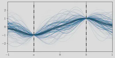
Note that the posterior mean is a sum of evaluations of the kernel scaled by $\fun{k}\call{\set{X}}^{-1} \vec{y}$. This shows that not only is the kernel important in the uncertainty estimation but that the interpolation and extrapolations capabilities of this posterior distribution is also dependent on the choice of kernel.
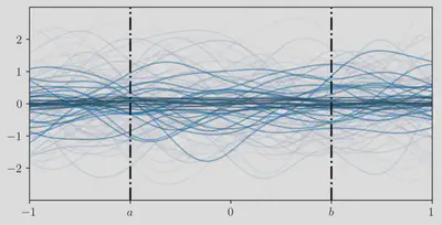
The most commonly used kernels, such as the squared exponential kernel or the Matérn family of kernels, belong to the class of stationary kernels. The defining property of stationary kernels is that all slices $\fun{k}(a,\blank)$ are the same: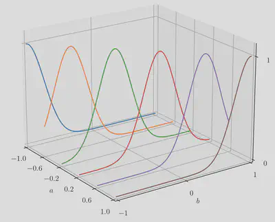
Nevertheless, it is known that this simple class of kernels is not enough to model and extrapolate interesting datasets. For example, many geospatial processes such as sea surface height, bathymetry and surface temperature are known to be non-stationary processes. Given the appeal of the simplicity of the stationary kernels, a productive research direction is to produce non-stationary kernels using these simple kernels as a base.
Non-stationary kernels from stationary
Let’s shortly review the terms surrounding stationary kernels. A kernel is stationary if: $$ \fun{k}\call{\vec{a}, \vec{b}} = \fun{k}\call{\vec{a}-\vec{b}, \vec{0}}. $$ This simplification means that stationary kernels don’t have an a priori preference for a specific position in space since they only depend on the relative distances between points.
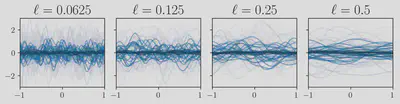
A further constrained class of kernels is the isotropic kernels: $$ \fun{k}\call{\vec{a}, \vec{b}} = \fun{\pi}_{\fun{k}}\call{\parens*{\vec{a}-\vec{b}}^{\T}\mat{\Delta}^{-1}\parens *{\vec{a}-\vec{b}}}. $$ These kernels depend only on the distance between two points, a further restriction from plain stationarity. These kernels are described by a scalar function $\fun{\pi}_{\fun{k}}$ and the positive semi-definite lengthscale matrix hyperparameter $\mat{\Delta}$. Usually this matrix is taken to be constant diagonal matrices $\mat{\Delta} = \ell^2\mat{I}$ or have each component of the diagonal be different. Nevertheless, it can be appropriate to learn the full matrix.
The very famous squared exponential kernel is an example of a stationary isotropic kernel, we simply take:
$$
\fun{\pi}_{\text{SE}}\call{d^2} = \exp\bcall{-\frac{1}{2}d^2}.
$$
Composition kernels
A very popular approach is to use a function to warp the inputs of the kernel, thus, even if the original kernel is stationary in the warped space, if we consider it as a function of the original space, the function can be non-stationary.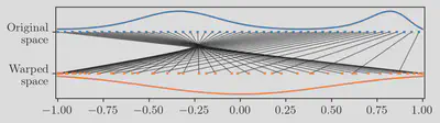
Given a warping function $\vecfun{\tau}\call\blank$, we express this class of kernels as: $$ \fun{k}_{\vecfun{\tau}}\call{\vec{a},\vec{b}} = \fun{k}\call{\vecfun{\tau}\call{\vec{a}}, \vecfun{\tau}\call{\vec{b}}} $$ The expressiveness of this composite kernel is strongly dependent on the type of warping function. For example, deforming an isotropic kernel linearly $\fun{\tau}\call{x} = \ell^{-1}\cdot x$ only changes the lengthscale of the kernel.
If we use a neural network as our warping function, this is the method described by deep kernel learning (DKL) 1.
However, if we instead use a Gaussian process prior on $\vecfun{\tau}\call\blank$, we can build a hierarchical GP model where each layer is the warping function of the next’s layer. This is the proposal in deep GPs 2 which we will refer as compositional deep GP (CDGP), in order to distinguish it from other hierarchical GP models.
Limitations
The main limitation of this approach is that isotropic kernels have very interpretable hyperparameters, however, for compositional kernels, the interpretability bottleneck is placed on the warping function instead. So, very expressive warping functions like neural networks eliminate the attractiveness of kernel methods.
More specifically, for this DKL case, since the warping function is not Bayesian, the large number of parameters negate most benefits of the GP Bayesian inference, including protection from overfitting.
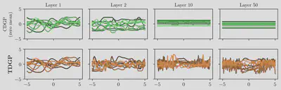
Meanwhile, for CDGPs, since the incentive with compositional kernels is to potentially compress high dimensional data, it would be interesting to place a zero mean prior on the transformation $\vecfun{\tau}\call\blank$ to incentivise the latent space to more sparse. However, with the increase of depth, these models quickly collapse and can’t be used for learning 3. Therefore, in practice, most models use other mean functions 4.
Lengthscale mixture kernels
Alternatively, instead of warping the input space, some authors explored ways to make the lengthscale hyperparameter $\mat{\Delta}$ vary along the input space. The most popular approach is defined as follows:5
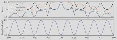
\begin{align} \fun{k}_{\matfun{\Delta}}\call{\vec{a},\vec{b}} =& \sqrt{\frac{ \sqrt{\det{\matfun{\Delta}\call{\vec{a}}}}\sqrt{\det{\matfun{\Delta}\call{\vec{b}}}} }{ \det{\frac{\matfun{\Delta}\call{\vec{a}}+\matfun{\Delta}\call{\vec{b}}}{2}} }}\;\times\\ &\fun{\pi}_{\fun{k}}\call{\parens*{\vec{a}-\vec{b}}^{\T}\bracks*{ \frac{\matfun{\Delta}\call{\vec{a}}+\matfun{\Delta}\call{\vec{b}}}{2} }^{-1}\parens*{\vec{a}-\vec{b}}}, \end{align} where the upper term is called the “pre-factor”.
In the case where the base kernel is the square exponential, this kernel is known as Gibbs’ kernel, as Mark Gibbs first derived this kernel 6.
To build hierarchical models using this kernel, it is enough to specify a function of positive semi-definite matrices $\matfun{\Delta}\call\blank$. In the context of GPs, this can be achieved by using a function $\fun{\sigma}\call\blank$ which warps the GP output from a Gaussian distribution to a distribution with positive semi-definite matrices as support. Thus, a hierarchical model like deeply non-stationary Gaussian process 7 is defined.
The main benefit in interpretability of methods like this compared to traditional compositional models like DKl and CDGP is that each lengthscale function is always a function of the input space and not of a previously deformed space. Therefore, all elements in the hierarchy can be inspected in terms of the original space and each of them control the interpretable lengthscales of the next layer.
 for the stationary case.](/blog/2024-tdgp/plots/mixture2_hu6b1ad6d5c9c7e7529115d74e699dac2e_407578_ac2f59b8e83a33f50a7085fd6c15d7b2.webp)
Limitations
As observed by Paciorek 5 and Gibbs 6, the pre-factor term can be hard to interpret and lead to intuitive correlations, specially when there are sharp differences between the lengthscales being compared.
Additionally, as the quadratic term that gets sent to $\fun{\pi}_{\fun{k}}$ doesn’t define a proper metric space, it is unknown if these kernels can be expressed in terms of latent spaces, thus, losing the benefits of learning lower-dimensional embeddings of data.
Our hybrid proposal
Returning to the compositional kernels, we observed that given a stationary kernel, linear deformations only correspond to changes in lengthscale. More explicitly, consider a linear deformation of a square exponential kernel: \begin{align} \fun{k}_{\vecfun{\tau}}\call{\vec{a},\vec{b}} &= \exp\bcall{-\frac{1}{2}\parens*{\vecfun{\tau}\call{\vec{a}}-\vecfun{\tau}\call{\vec{b}}}^\T\parens*{\vecfun{\tau}\call{\vec{a}}-\vecfun{\tau}\call{\vec{b}}}}\\ &= \exp\bcall{-\frac{1}{2}\parens*{\mat{W}{\vec{a}}-\mat{W}{\vec{b}}}^\T\parens*{\mat{W}{\vec{a}}-\mat{W}{\vec{b}}}}\\ &= \exp\bcall{-\frac{1}{2}\parens*{{\vec{a}}-{\vec{b}}}^\T\bcall{\mat{W}^\T\mat{W}}\parens*{{\vec{a}}-{\vec{b}}}}, \end{align} therefore, in this case, the lengthscales of the deformed kernel are $\bracks*{\mat{W}^\T\mat{W}}^{-1}$.
Our proposal is to expand to take this deformation and turn it into a locally linear deformation $\vecfun{\tau}\call{\vec{x}} = \matfun{W}\call{\vec{x}}\,\vec{x}$. Using this deformation, we can use it to define a lengthscale field $\matfun{\Delta}\call{\vec{x}} = \bracks*{\matfun{W}^\T\call{\vec{x}}\matfun{W}\call{\vec{x}}}^{-1}$ while reaping the benefits of learning latent spaces. This $\matfun{W}\call\blank$ can be directly parametrized with a Gaussian process since there is no restrictions on its entries, unlike for the lengthscale function $\matfun{\Delta}\call\blank$.
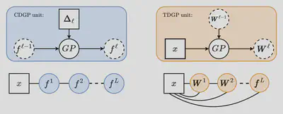
To propose a hierarchical GP using this type of kernel transformation, we propose keeping the deformation rooted in the original input space but composing the weight matrix normally. In other words, a two layer deep deformation has form: \begin{align} \vecfun{\tau}^{(1)}\call{\vec{x}} &= \matfun{W}^{(1)}\call{{\vec{x}}}\,\vec{x}\\ \vecfun{\tau}^{(2)}\call{\vec{x}} &= \matfun{W}^{(2)}\call{\vecfun{\tau}^{(1)}\call{\vec{x}}}\,\vec{x}\\ &= \matfun{W}^{(2)}\call{ \matfun{W}^{(1)}\call{\vec{x}}\,\vec{x} }\,\vec{x}, \end{align} with the prior distributions: \begin{align} \matfun{W}^{(1)}\call\blank &\sim \prod_{i,j} \operatorname{GP}\parensgiven*{\fun{w}^{(1)}_{ij}}{\fun{0}, \fun{k}}\\ \matfun{W}^{(2)}\call\blank &\sim \prod_{i,j} \operatorname{GP}\parensgiven*{\fun{w}^{(2)}_{ij}}{\fun{0}, \fun{k}_{\vecfun{\tau}^{(1)}}}\\ \fun{f}\call\blank &\sim \GPdist{\fun{0}, \fun{k}_{\vecfun{\tau}^{(2)}}}. \end{align} Therefore, each node in the hierarchical model is still connected to the input layers, just like in DNSGP but not in the traditional CDGP. Fig. 9 shows a graphical representation. For this reason, we name our proposal thin and deep Gaussian processes, as the size of the smallest loop (i.e. its girth) is always 3, instead of the unbounded girth of the traditional CDGP model.
Variational inference
As with any deep GP model, the posterior distribution is not a Gaussian process and approximate inference has to be used. For this work, we choose to apply the variational inference with inducing points framework that’s common used for deep GPs 24. We introduce $m_{\ell}$ inducing points for each layer $\ell$, such that our variational posterior distribution is: \begin{alignat}{3} &p\callgiven{\fun{f}}{\matfun{W}^{(L)}, \vec{u}^{(L+1)}} &&&&q\call{\vec{u}^{(L+1)}}\\ \prod_{\ell=2}^L &p\callgiven{\matfun{W}^{(\ell)}}{\matfun{W}^{(\ell-1)}, \mat{V}^{(\ell)}} &&\prod_{d,q}^{D,Q_{\ell}}&&q\call{\vec{v}_{: dq}^{(\ell)}}\\ &p\callgiven{\matfun{W}^{(1)}}{\mat{V}^{(1)}} &&\prod_{d,q}^{D,Q_1}&&q\call{\vec{v}_{:dq}^{(1)}}, \end{alignat} where the $q$ distributions are parametrized by a mean and covariance vectors of dimension $m_{\ell}$. By exploiting earlier results from VI on square exponential hyperparameters 8, we propose a deterministic closed-form VI scheme restricted when the base kernel $\fun{\pi}_{\fun{k}}$ is restricted to squared exponential. Nevertheless, we can use doubly stochastic inference 4 to remove this restriction at the cost of having to estimate the ELBO.
Limitations
The biggest drawback of the kernel that we propose is that by deforming the space with locally linear transformations is that the neighbourhood around $0$ is not affected by linear transformations, unlike CDGP or DNSGP. A possible solution is to add a bias term to the input data and effectively turning local linear transforms into affine transforms that do not preserve the neighbourhood around $0$.
A limitation that comes with the hierarchical GP approach is the increased number of output channels in each GP layer of the TDGP architecture. More specifically, for the compositional DGP, to learn a latent space with dimension $Q$, it requires a GP layer with output dimension $Q$, however, for TDGP, we require output dimension $Q\times D$, as we learn the transformation matrix.
Results in geospatial datasets
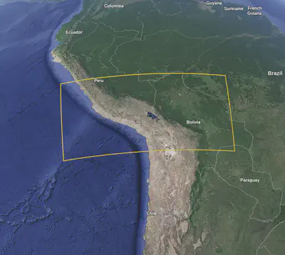
As a case-study, we also apply TDGP to the GEBCO gridded bathymetry dataset. It contains a global terrain model (elevation data) for ocean and land. We selected an especially challenging subset of the data covering the Andes mountain range, ocean, and land.
This region was subsampled to 1,000 points from this region and compared with the methods via five-fold cross validation. The baselines chosen are: single layer sparse GP 9, stochastic variational DKL 1, doubly stochastic deep GP 4, and deeply stationary GP 7.
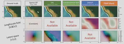
As seen in the results plot, TDGP is the only method that learns both a lengthscale field, represented as the trace of the lengthscale matrix, and a latent space, represented with a domain colored plot. Not only that, but we can see that the regions of lower lengthscale are well correlated with higher spatial variance.
| NLPD | MRAE | |
|---|---|---|
| Sparse GP | -0.13 ± 0.09 | 1.19 ± 0.63 |
| Deep Kernel Learning | 3.85 ± 0.92 | 0.59 ± 0.31 |
| Compositional DGP | -0.44 ± 0.12 | 0.83 ± 0.56 |
| TDGP (Ours) | -0.53 ± 0.10 | 0.66 ± 0.43 |
In terms of metrics, our proposal has the best negative log predictive density, showing that our predictions are well calibrated, and only losing to DKL in terms of mean error. However, our method has the best balance between the accuracy of the mean and uncertainty calibration.
Conclusion
We’ve introduced Thin and Deep Gaussian Processes (TDGP), a new hierarchical architecture for DGPs. TDGP’s strength lies in its ability to recover non-stationary functions through locally linear deformations of stationary kernels, while also learning lengthscale fields. Unlike regular compositional DGPs, TDGP sidesteps the concentration of prior samples that happens with increasing layers. Our experiments confirm TDGP’s strengths in tasks with latent dimensions and geospatial data.
We hope to investigate further how the more interpretable hidden layers can be used with addition of expert knowledge, either in the prior or in the variational posterior, and apply this method in areas where models like DNSGP couldn’t be applied, due to the lack of latent space embeddings.
References
Andrew Gordon Wilson, Zhiting Hu, Ruslan Salakhutdinov, Eric P. Xing. “Stochastic Variational Deep Kernel Learning” (2016) ↩︎ ↩︎
Andreas C. Damianou, Neil D. Lawrence “Deep Gaussian Processes” (2013) ↩︎ ↩︎
David Duvenaud, Oren Rippel, Ryan Adams, and Zoubin Ghahramani “Avoiding pathologies in very deep networks” (2014) ↩︎
Hugh Salimbeni, Marc Peter Deisenroth. “Doubly Stochastic Variational Inference for Deep Gaussian Processes” (2017) ↩︎ ↩︎ ↩︎ ↩︎
Christopher J. Paciorek, Mark J. Schervish “Nonstationary Covariance Functions for Gaussian Process Regression” (2003) ↩︎ ↩︎
Mark N. Gibbs “Bayesian Gaussian Processes for Regression and Classification” (1997) ↩︎ ↩︎
Hugh Salimbeni, Marc Peter Deisenroth. “Deeply Non-Stationary Gaussian Processes” (2017) ↩︎ ↩︎
Michalis K. Titsias, Miguel Lázaro-Gredilla. “Variational Inference for Mahalanobis Distance Metrics in Gaussian Process Regression” (2013) ↩︎
Michalis K. Titsias “Variational Learning of Inducing Variables in Sparse Gaussian Processes” (2009) ↩︎