Iterative State Estimation in Non-linear Dynamical Systems Using Approximate Expectation Propagation

State estimation in nonlinear systems is difficult due to the non-Gaussianity of posterior state distributions. For linear systems, an exact solution is attained by running the Kalman filter/smoother. However for nonlinear systems, one typically relies on either crude Gaussian approximations by linearising the system (e.g. the Extended Kalman filter/smoother) or to use a Monte-Carlo method (particle filter/smoother) that sample the non-Gaussian posterior, but at the cost of more compute.

We propose an intermediate nonlinear state estimation method based on (approximate) Expectation Propagation (EP), which allows for an iterative refinement of the Gaussian approximation based on message passing. It turns out that this method generalises any standard Gaussian smoother such as the Extended Kalman smoother, in the sense that these well-known smoothers are special cases of (approximate) EP. Moreover, they have the same computational cost up to the number of iterations, making it a practical solution to improving state estimates.

State Estimation

The aim of state estimation is to provide an estimate of a time-evolving latent state based on noisy observations of the dynamical system. This can be formulated mathematically using the state-space model:

$$ x_t = f_{t-1}(x_{t-1}) + w_t, \quad t = 1, \ldots, T, $$

$$ y_t = h_t(x_t) + v_t, \quad t = 1, \ldots, T. $$

Here, $x_t$ is the latent state that we wish to estimate, with initial state distribution $x_0 \sim p(x_0)$ and transition function $f$ (the dynamical system that describe the evolution of the latent state). $y_t$ is the observation of $x_t$, obtained via an observation operator $h$. $w_t$ and $v_t$ are the model error and measurement error respectively, typically chosen to be Gaussians.

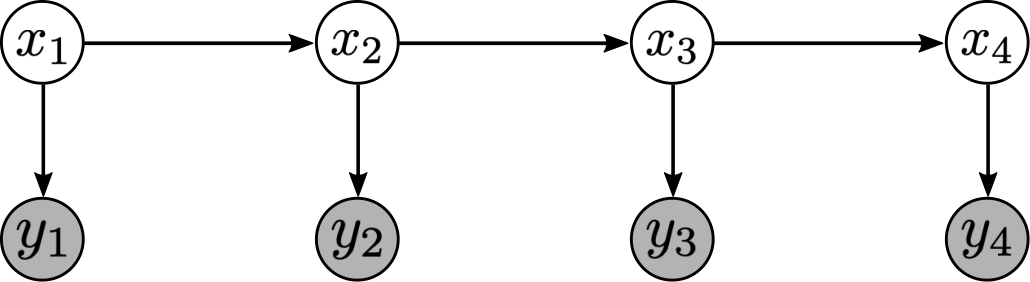
Figure 1. Graphical representation of a state-space model.

We distinguish between two types of solutions. In filtering, a solution to the state estimation problem is given by the probability distribution $p(x_t | y_1, \ldots, y_t)$ of the state $x_t$ conditioned on observations up to the current time $t$. On the other hand, smoothing yields the solution $p(x_t | y_1, \ldots, y_T)$, i.e. the distribution of state $x_t$ conditioned on all available observations up to time $T$. Here, we will mostly be concerned with smoothing.

Expectation propagation

Expectation propagation (EP)¹ gives us a way to approximate intractable distributions in a Bayesian network by simpler ones. Assuming that the (intractable) marginal factorises as

$$ p(x_t | y_{1:T}) = \prod_{i=1}^N f_i(x_t), $$

EP approximates this using a simpler distribution of the form $q(x_t) = \prod_i q_i(x_t)$, where the factors $q_i$ come from the exponential family $\mathcal{F}$, usually Gaussians. This is achieved by iterating the following three steps:

For every $i = 1, 2, \ldots, N$,

1. Form the cavity distribution:

$$ q_{\backslash i}(x_t) \propto q(x_t)/q_i(x_t). $$

2. Projection:

$$ q^{new}(\cdot) = \arg\min_{q \in \mathcal{F}} KL(f_i q_{\backslash i} || q). $$

3. Update factor:

$$ q_i^{new}(x_t) \propto q^{new}(x_t) / q_{\backslash i}(x_t). $$

When the KL-divergence in Step 2 is replaced by the $\alpha$-divergence, this is called Power EP². Moreover, we can consider a damped update

$$ q_i^{new}(x_t) = q^{new}(x_t)^\gamma q(x_t)^{1-\gamma} / q_{\backslash i}(x_t), $$

in Step 3 with damping factor $\gamma \in (0, 1]$, which can give better convergence behaviour (although convergence is not guaranteed).

Approximate EP for state-space models

For state-space models (Figure 1), the true marginal posterior on $x_t$ has the following decomposition

$$ p(x_t | y_{1:T}) = f_\rhd(x_t) f_\vartriangle(x_t) f_\lhd(x_t), $$

where the forward message

$$ f_\rhd(x_t) := \int p(x_t | x_{t-1}) f_\rhd(x_{t-1}) f_\vartriangle(x_{t-1}) d x_{t-1}, $$

carries information about past observations, the measurement message

$$ f_\vartriangle(x_t) := p(y_t | x_t), $$

incoorporates the measurement at the current timestep $t$, and the backward message

$$ f_\lhd(x_t) := \int p(x_{t+1} | x_{t}) f_\lhd(x_{t+1}) f_\vartriangle(x_{t+1}) d x_{t+1}, $$

brings in information about future observations.

Note that the forward ($\rhd$) and backward ($\lhd$) messages at time $t$ depend on messages on the neighbouring nodes (e.g. $f_\vartriangle(x_{t-1})$), making them difficult to evaluate. We overcome this difficulty in our approximate EP framework by replacing them with the corresponding approximate messages such as $q_\vartriangle(x_{t-1})$ that we iteratively refine in EP. These messages are assumed to be Gaussian for simplicity.

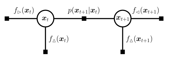
(a) Factor graph

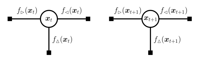
(b) Fully-factored factor graph

Figure 2. Messages in state-space models. We can run EP on each node by decomposing the (a) factor graph as a (b) fully-factored factor graph.

We can now run the EP algorithm with these approximated ‘’true’’ messages $f_i(x_t), i \in \{\rhd, \vartriangle, \lhd\}$ to update the approximating messages $q_i(x_t), i \in \{\rhd, \vartriangle, \lhd\}$ for all $t = 1, \ldots, T$.

In practice, the projection step in EP cannot be solved exactly when the true messages $f_i(x_t)$ are non-Gaussian, as is the case here. To this end, we further approximate the messages by linearising the transition function $f_t$ and measurement function $h_t$ either explicitly (i.e., Taylor expansion), or implicitly, e.g. using an unscented transform, which makes this projection step tractable.

Choice of EP schedule

While we can update the nodes in any order we wish, we typically update them in a forward-backward sweep, where we first update $q(x_t)$ for $t$ going from $1$ to $T$ (ascending order), and once complete, re-update $q(x_t)$ for $t$ now going from $T$ to $1$ (descending order). This is a sensible choice due to the sequential nature of the problem. It is also possible to update the nodes all at once in a distributed manner to further speed up computations, although we do not investigate this here.

Strategies to improve state estimates

With the approximations made above, we prove the following key result:

Theorem. Any nonlinear Gaussian smoother is equivalent to a single forward-backward iteration of approximate EP as described above.

This generalises the well-known result of the equivalence between Kalman smoother and EP for linear systems. However, while for linear systems, a single iteration of EP (and hence the Kalman smoother) already gives the optimal solution and further iterations do not improve the result, for nonlinear systems, the first iteration is far from optimal. Iterating EP may therefore give better results, since the fixed points of EP correspond to the minima of the Bethe free energy^{3 4}.

There are still problems however since the EP algorithm is not guaranteed to converge. To remedy this, damped updates can be applied to help the algorithm converge. In addition, by using power EP instead of EP, one can make the predictions more mode-seeking, which can also improve results.

Examples

Below, we showcase the results of iterated approximate damped-power EP on some benchmarks.

Uniform Nonlinear Growth Model

The uniform nonlinear growth model (UNGM) is a well-known 1D nonlinear benchmark for state estimation, given as follows.

$$ f_t(x) = \frac{x}{2} + \frac{25 x}{1 + x^2} + 8 \cos(1.2t), \qquad h_t(x) = \frac{x^2}{20}. $$

The video below shows the result of EP iterations with the following setup.

• Linearisation method: unscented transform
• Power: $\alpha = 0.9$
• Damping: $\gamma = 0.4$
• Number of iterations: 50

Figure 3. Iterating damped power EP improves smoother results for the uniform nonlinear growth model.

Bearings Only Tracking of a Turning Target

Next, we demonstrate our algorithm on the problem of bearings-only tracking of a turning target. This is a five dimensional nonlinear system in the variables $(x_1, \dot{x}_1, x_2, \dot{x}_2, \omega)$. We use the following setup for EP iterations:

• Linearisation method: Taylor transform
• Power: $\alpha = 1.0$
• Damping: $\gamma = 0.6$
• Number of iterations: 10

Figure 4. Damped EP applied to the bearings-only tracking problem. We only display the spatial components $(x_1, x_2)$. The green dots represent the predictive mean and the ellipses represent the spatial covariance.

Lorenz 96 Model

The Lorenz 96 model is another well-known benchmark for nonlinear state-estimation. This is governed by the following system of ODEs:

$$ \frac{\mathrm{d} x_i}{\mathrm{d} t} = (x_{i+1} - x_{i-2}) x_{i-1} - x_i + F, $$

for $i = 1, \ldots, d$. We consider a system with $F = 8$ and $d = 200$. The ODE is discretised using the fourth-order Runge-Kutta scheme. For the observation, we use the quadratic function $h(x) = x^2$ applied to each component. The following configurations are used for EP iteration:

• Linearisation method: unscented transform
• Power: $\alpha = 1.0$
• Damping: $\gamma = 1.0$
• Number of iterations: 5

Figure 5. Hovmöller representation of a single simulation of the L96 model. The absolute error of the EP prediction, and componentwise negative log likelihood loss are displayed.

References

Thomas P. Minka. Expectation Propagation for Approximate Bayesian Inference. In Proceedings of the Conference on Uncertainty in Artificial Intelligence, 2001. ↩︎
Thomas P. Minka. Power EP. Technical Report MSR-TR-2004-149, Microsoft Research, 2004. ↩︎
Heskes, Tom, and Onno Zoeter. Expectation propagation for approximate inference in dynamic bayesian networks. Proceedings of the Eighteenth conference on Uncertainty in artificial intelligence, 2002. ↩︎
This argument is only heuristic as we have made approximations to EP; the fixed points of approximate EP will not necessarily coincide with the fixed points of the Bethe free energy. ↩︎