Gaussian processes are machine learning models capable of learning unknown functions with uncertainty. Motivated by a desire to deploy Gaussian processes in novel areas of science, we present a new class of Gaussian processes that model random vector fields on Riemannian manifolds that is (1) mathematically sound, (2) constructive enough for use by machine learning practitioners and (3) trainable using standard methods such as inducing points. In this post, we summarize the paper and illustrate the main results and ideas.

Vector fields on manifolds

Before discussing Gaussian processes, we first review vector fields on manifolds. Let $X$ be a manifold—a smooth geometric space where the rules of calculus apply. For each $x \in X$, let $T_x X$ be the tangent space at $x$, which is a vector space intuitively representing all the directions one can move on the manifold from that point. The tangent bundle $TX$ is defined by gluing together all tangent spaces—this space is also a manifold. Let $\operatorname{proj}_X : TX \to X$ be the projection map, which takes vectors in the tangent space, and maps them back to the underlying points they are attached to. A vector field is a function $f: X \to TX$ satisfying the section property $f \circ \operatorname{proj}_X = \operatorname{id}_X$, meaning that the arrow $f(x) \in TX$ must be attached to the point $x$. We denote the space of vector fields by $\Gamma(TX)$.

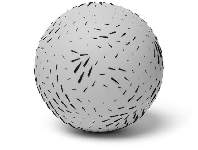
Vector fields reflect the topological properties of the manifolds they are defined on. For example, by the Poincaré–Hopf Theorem, there does not exist a smooth non-vanishing vector field on the sphere. This result is also known as the hairy ball theorem, because if we imagine a ball with hair attached to it, the result says we cannot comb the hair, making it tangential to the sphere, without creating a discontinuous cowlick. Note that, unlike in the Euclidean setting, this implies that a smooth vector field generally cannot be written as a continuous function $f : X \to \mathbb{R}^d$, and we must work with the machinery of tangent bundles to make sense of vector fields.

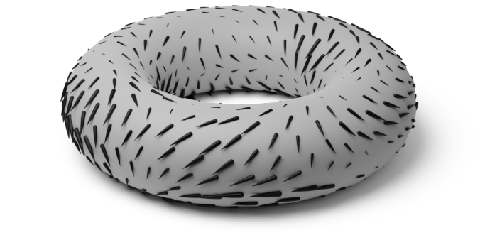
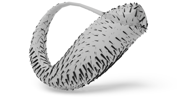
Examples of Gaussian random vector fields on the torus (left) and the Klein bottle (right).

Gaussian vector fields

To define Gaussian processes which are random vector fields, the first issue we must address is that a Gaussian process, classically, is a vector-valued random function $f : X \to \mathbb{R}^d$¹ which is, for any finite collection of points, Gaussian-distributed. However, a well-defined vector field is instead a random function $f : X \to TX$¹ satisfying the section property, and the range of this function is a manifold rather than a vector space, so it is not immediately clear in what sense such a function could be Gaussian. Therefore, the first step is to say what we actually mean by the term Gaussian in this setting.

Definition: A random vector field $f \in \Gamma(TX)$¹ is Gaussian if for any points $x_1, \ldots, x_n \in X$ on the manifold, the vectors $f(x_1),..,f(x_n) \in T_{x_1} X \oplus .. \oplus T_{x_n} X$ attached to it are jointly Gaussian.

Here, $\oplus$ is the direct sum of vector spaces. With this definition in place, our next step is to show that standard properties of Gaussian processes carry over to this setting. In particular, we would like to characterize Gaussian vector fields in terms of a mean function and a covariance kernel. The former notion is clear: the mean of a Gaussian vector field should just be an ordinary vector field that will determine the mean vector at all finite-dimensional marginals. On the other hand, generalizing matrix-valued kernels is less obvious, as it is not clear what the appropriate notion of a matrix should be in the geometric setting.

The covariance kernel of a Gaussian vector field

To generalize the notion of a matrix-valued kernel to the geometric setting, we introduce the following definition.

Definition. We say that a scalar-valued function $k : T^*X \times T^*X \to \mathbb{R}$ is a cross-covariance kernel if it satisfies the following key properties.

1. Symmetry: for all $\alpha, \beta \in T^*X$, $k(\alpha, \beta) = k(\beta, \alpha)$ holds.
2. Fiberwise bilinearity: for any pairs of points $x, x’ \in X$, $k(\lambda \alpha_x + \mu \beta_x, \gamma_{x’}) = \lambda k(\alpha_x, \gamma_{x’}) + \mu k(\beta_x, \gamma_{x’})$ holds for any $\alpha_x, \beta_x \in T^x X$, $\gamma{x’} \in T^_{x’} X$ and $\lambda, \mu \in \mathbb{R}$.
3. Positive definiteness: for any $\alpha_1, .., \alpha_n \in T^*X$, we have $\sum_{i=1}^n\sum_{j=1}^n k(\alpha_i, \alpha_j) \geq 0$.

Here, $T^* X$ is the cotangent bundle, which is constructed similarly to the tangent bundle, but by gluing together the dual of the tangent spaces $(T_x X)^*$ instead of the tangent spaces. Why is this definition precisely the notion we need? In this work, we prove that cross-covariance kernels in the above sense are exactly analogous to Euclidean matrix-valued kernels.

Theorem. Every Gaussian random vector field admits and is uniquely determined by a mean vector field and a cross-covariance kernel.

Projected kernels

The preceding ideas tell us what a Gaussian vector field is, but say little about how to implement one numerically. To proceed towards this, we rely on an extrinsic geometric approach we call the projected kernel construction. This is detailed as follows.

1. Embed the manifold isometrically into a higher-dimensional Euclidean space $\mathbb{R}^{d’}$.²

2. Construct a vector-valued Gaussian process $\boldsymbol{f} : X \rightarrow \mathbb{R}^{d’}$ in the usual sense with a matrix-valued kernel $\boldsymbol{\kappa} : X \times X \rightarrow \mathbb{R}^{d’} \times \mathbb{R}^{d’}$.

3. Project the vectors of the resulting function so that they become tangential to the manifold, giving a vector field.

In this work, we show that (1) this procedure defines a cross-covariance kernel, and (2) all cross-covariance kernels arise this way and therefore no expressivity is lost by employing this construction. Thus, once we have a matrix-valued kernel $\boldsymbol{\kappa} : X \times X \rightarrow \mathbb{R}^{d’} \times \mathbb{R}^{d’}$ taking values in the higher dimensional Euclidean space, we obtain completely general workable kernels for Gaussian random vector fields. Constructing such matrix-valued kernels, in turn, can be done for example by using scalar-valued Riemannian Gaussian processes³ as building blocks.

By connecting differential-geometric cross-covariance kernels with Euclidean matrix-valued kernels, we can carry over standard Gaussian process techniques, such as variational approximations, into the differential-geometric setting. Here, we show how to check such approximations to ensure they are geometrically consistent,⁴ and show in particular that the classical inducing point framework⁵ satisfies this. This allows us to use variational approximations directly out of the box, with almost no modification to the code.

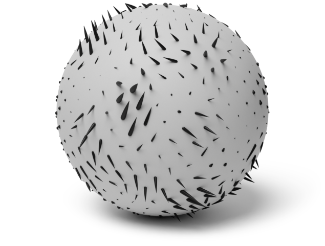
We illustrate this general procedure below. Here, three scalar processes are combined to create a non-tangential vector-valued process in the embedded space, and projected to obtain a tangential vector field on the manifold.

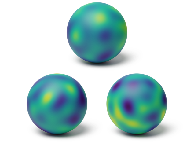
(a) Scalar processes

(b) Embedded process

(c) Projected process

Illustration of Gaussian processes constructed using projected kernels.

Example: probabilistic global wind interpolation

Here, we demonstrate a simplified example of the developed model on the problem of interpolating the global wind field from satellite observations. We focus on the benefit of using a geometrically consistent model over a naïve implementation using Euclidean Gaussian processes. Results are shown below.

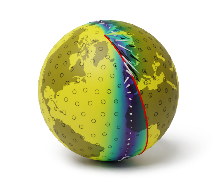
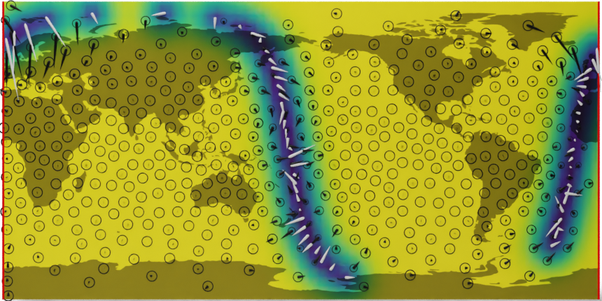
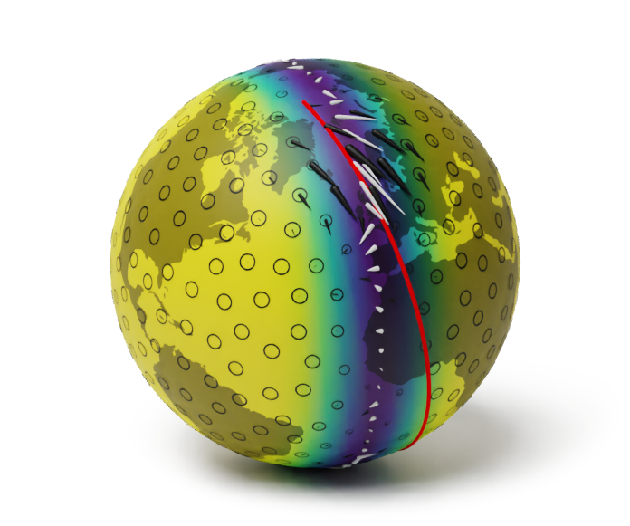
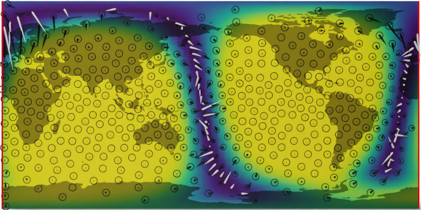
Wind interpolation using a Euclidean process (top) and Riemannian process (bottom).

We see that the uncertainties in the Euclidean vector-valued GP become unnaturally distorted as the satellite approaches the poles, while the Riemannian case has a uniform band along the observations. In addition, the Euclidean process gives rise to a spurious discontinuity in the uncertainty along the solid red line, which indicates the latitudinal boundary when projected onto the plane. Such artifacts are avoided with a geometrically consistent model.

Summary

We have developed techniques that enable Gaussian processes to model vector fields on Riemannian manifolds by providing a well-defined notion of such processes and then introducing an explicit method to construct them. In addition to this, we have seen that most standard Gaussian process training methods, such as variational inference, are compatible with the geometry, hence can be used safely within our framework. In an initial demonstration of our technique on the wind observation data, we have shown that it can be used successfully to interpolate global wind field with geometrically consistent uncertainty bars. We hope that our work inspires the use of Gaussian processes as easy and flexible means of modelling vector fields on manifolds in a variety of applications.

References