Matérn Gaussian Processes on Riemannian Manifolds

Gaussian processes are a useful technique for modeling unknown functions. They are used in many application areas, particularly in cases where quantifying uncertainty is important, such as in strategic decision-making systems. We study how to extend this model class to model functions whose domain is a Riemannian manifold, for example, a sphere or cylinder. We do so in a manner which is (a) mathematically well-posed, and (b) constructive enough to allow the kernel to be computed, thereby allowing said processes to be trained with standard methods. This in turn enables their use in Bayesian optimization, modeling of dynamical systems, and other areas.

Matérn Gaussian processes

One of the most widely-used kernels is the Matérn kernel, which is given by $$ k(x,x’) = \sigma^2 \frac{2^{1-\nu}}{\Gamma(\nu)} \left(\sqrt{2\nu} \frac{||x-x’||}{\kappa}\right)^\nu K_\nu \left({\sqrt{2\nu} \frac{||x-x’||}{\kappa}}\right) $$ where $K_\nu$ is the modified Bessel function of the second kind, and $\sigma^2,\kappa,\nu$ are the variance, length scale, and smoothness parameters, respectively. As $\nu\to\infty$, the Matérn kernel converges to the widely-used squared exponential kernel.

To generalize this class of Gaussian processes to the Riemannian setting, one might consider replacing Euclidean distances $||x-x’||$ with the geodesic distance $d_g(x, x’)$. Unfortunately, this doesn’t necessarily define a valid kernel: in particular, the geodesic squared exponential kernel already fails to be positive semi-definite for most manifolds, due to a recent no-go result.¹² We therefore adopt a different approach, which is not based on geodesics.

Stochastic partial differential equations

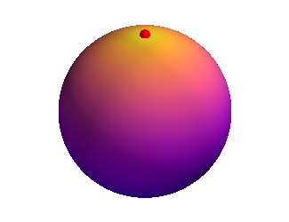
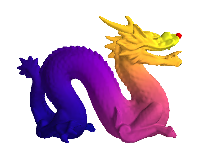
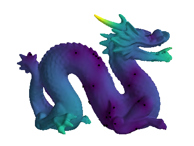
Whittle³ has shown that Matérn Gaussian processes satisfy the stochastic partial differential equation $$ \left({\frac{2 \nu}{\kappa^2} - \Delta}\right)^{\frac{\nu}{2} + \frac{d}{4}}f = \mathcal{W} $$ where $\Delta$ is the Laplacian, and $\mathcal{W}$ is Gaussian white noise.⁴ This gives another way to generalize Matérn Gaussian processes from the Euclidean to the Riemannian setting: replace the Laplacian and white noise process with their Riemannian analogues. The kernels of these processes, calculated via our technique on three example manifolds, namely, the circle, sphere, and dragon, are shown below, where color represents the value of the kernel between any given point and the red dot.

Unfortunately, this process is somewhat non-constructive: to train such Gaussian processes on data, one resorts to solving these SPDEs,⁵ which without further modifications needs to be done repeatedly for every posterior sample, which can become rather involved, particularly if the chosen smoothness $\nu$ yields SPDEs of fractional order. In this work, we compute workable expressions for the kernels of these processes, so they can be used by practitioners without detailed knowledge of SPDEs.

An expression for the kernel through Laplace–Beltrami eigenfunctions

A Riemannian manifold’s geometry can be quite complicated, so there is no hope of an entirely closed-form expression for the kernel in general. We therefore focus on workable expressions in terms of computable geometric quantities on the manifold, restricting ourselves to compact Riemannian manifolds without boundary. In this setting, the eigenvalues $\lambda_n$ and eigenfunctions $f_n$ of the Laplace–Beltrami operator $\Delta_g$ are countable, and form an orthonormal bases. We prove that the kernel of a Riemannian Matérn Gaussian process is given by $$ k(x,x’) = \frac{\sigma^2}{C} \sum_{n=0}^\infty \left({\frac{2 \nu}{\kappa^2} + \lambda_n}\right)^{-\nu + \frac{d}{2}} f_n(x) f_n(x’) $$ where $C$ is a constant chosen so that the variance is $\sigma^2$ on average.⁴ By truncating this sum, we obtain a workable approximation for the kernel,⁶ allowing us to train the process on data using standard methods, such as sparse inducing point techniques.⁷⁸ The resulting posterior Gaussian processes are visualized below.

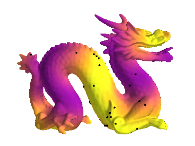
(a) Ground truth

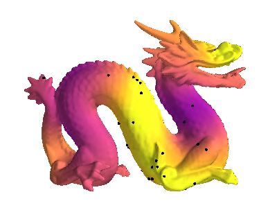
(b) Posterior mean

(c) Standard deviation

The Laplace–Beltrami eigenvalues $\lambda_n$ and eigenfunctions $f_n$ are analytic in many cases of interest, such as the sphere, but it’s also possible to compute them numerically by solving a Helmholtz equation. This equation is very well-studied, and a number of scalable techniques for solving it exist, owing to its use throughout mathematics, engineering, and computer graphics.

Concluding remarks

We present techniques for computing the kernels, spectral measures, and Fourier feature approximations of Riemannian Matérn and squared exponential Gaussian processes, using spectral techniques via the Laplace–Beltrami operator. This allows us to train these processes via standard techniques, such as variational inference via sparse inducing point methods,⁷⁸ or Fourier feature methods.⁹ In turn, this allows Riemannian Matérn Gaussian processes to easily be deployed in mini-batch, online, and non-conjugate settings. We hope this work enables practitioners to easily deploy techniques such as Bayesian optimization in this setting.

References

A. Feragen, F. Lauze, and S. Hauberg. Geodesic exponential kernels: When curvature and linearity conflict. CVPR, 2015. ↩︎
A. Feragen and S. Hauberg. Open problem: Kernel methods on manifolds and metric spaces: what is the probability of a positive definite geodesic exponential kernel? COLT, 2016. ↩︎
P. Whittle. Stochastic processes in several dimensions. Bulletin of the International Statistical Institute 40(2):974–994, 1963. ↩︎
A similar expression is also available for the limiting squared exponential case. ↩︎ ↩︎
F. Lindgren, H. Rue, and J. Lindström. An explicit link between Gaussian fields and Gaussian Markov random fields: the stochastic partial differential equation approach. JRSSB, 73(4):423–498, 2011. ↩︎
A similar expression is also available for the spectral measure. ↩︎
M. Titsias. Variational learning of inducing variables in sparse Gaussian processes. AISTATS, 2009. ↩︎ ↩︎
J. Hensman, N. Fusi, N. Lawrence. Gaussian Processes for Big Data. UAI, 2013. ↩︎ ↩︎
A. Rahimi and B. Recht. Random features for large-scale kernel machines. NeurIPS, 2008. ↩︎